How to break regression
 Photo illustration by Pew Research Center and iStock.com/Eshma
Regression models are a cornerstone of modern social science. They’re at the heart of efforts to estimate causal relationships between variables in a multivariate environment and are the basic building blocks of many machine learning models. Yet social scientists can run into a lot of situations where regression models break.
Famed social psychologist Richard Nisbett recently argued that regression analysis is so misused and misunderstood that analyses based on multiple regression “are often somewhere between meaningless and quite damaging.” (He was mainly talking about cases in which researchers publish correlational results that are covered in the media as causal statements about the world.)
Below, I’ll walk through some of the potential pitfalls you might encounter when you fire up your favorite statistical software package and run regressions. Specifically, I’ll be using simulation in R as an educational tool to help you better understand the ways in which regressions can break.
Using simulations to unpack regression
The idea of using R simulations to help understand regression models was inspired by Ben Ogorek’s post on regression confounders and collider bias.
The great thing about using simulation in this way is that you control the world that generates your data. The code I’ll introduce below represents the true data-generating process,since I’m using R’s random number generators to simulate the data. In real life, of course, we only have the data we observe, and we don’t really know how the data-generating process works unless we have a solid theory (like Newtonian physics or evolution) where the system of relevant variables and causal relationships is well understood and to which there is really no analogous phenomenon in social science.
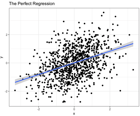
What I’ll do here is create a dataset based on two random standard normal variables by simulating them using the rnorm() function, which draws random values from a normal distribution with mean 0 and standard deviation 1, unless you specify otherwise. I’ll create a functional relationship between y and x such that a 1 unit increase in x will be associated with a .4 unit increase in y.
# make the code reproducible by setting a random number seed
set.seed(100)

# When everything works:
N <- 1000
x <- rnorm(N)
y <- .4 * x + rnorm(N)
hist(x)
hist(y)

# Now estimate our model:
summary(lm(y ~ x))

Call:
lm(formula = y ~ x)
Residuals:
    Min      1Q  Median      3Q     Max
-3.0348 -0.7013  0.0085  0.6212  3.1688
Coefficients:
            		Estimate Std. Error t value Pr(>|t|)
(Intercept) 	0.003921   0.031039   0.126    0.899
x           	0.413415   0.030129  13.722   <2e-16 ***
---
Signif. codes:  0 ‘***’ 0.001 ‘**’ 0.01 ‘*’ 0.05 ‘.’ 0.1 ‘ ’ 1
Residual standard error: 0.9814 on 998 degrees of freedom
Multiple R-squared:  0.1587,	Adjusted R-squared:  0.1579
F-statistic: 188.3 on 1 and 998 DF,  p-value: < 2.2e-16

# Plot it
library(ggplot2)
qplot(x, y) +
  geom_smooth(method='lm') +
  theme_bw() +
  ggtitle("The Perfect Regression")
Notice that the model estimates the functional relationship between x and y that I simulated quite well. The plot looks like this:
What about omitted variables? Our machinery actually still works if there is another factor causing y, as long as it is uncorrelated with x.
The dreaded omitted variable bias
Omitted variable bias (OVB) is much feared, and judging by the top internet search results, not well understood. Some top sources say it occurs when “an important” variable is missing or when a variable that “is correlated” with both x and y is missing. I even found a university econometrics course that defined OVB this way.
But neither of those definitions are quite right. OVB occurs when a variable that causes y is missing from the model (and is correlated with x). Let’s call that variable w. Because w is in play when we consider the causal relationship between x and y, it’s often referred to as “endogenous” or a “confounding variable.”
The example below first demonstrates that w, our confounding variable, will bias our results if we fail to include it in our model. The next two examples are essentially a re-telling of the post I mentioned above on collider bias, but emphasizing slightly different points.
w <- rnorm(N)
x <- .5 * w + rnorm(N)
y <- .4 * x + .3 * w + rnorm(N)

m1 <- lm(y ~ x)
summary (m1) # Omitted variable bias

Call:
lm(formula = y ~ x)

Residuals:
    Min      1Q  Median      3Q     Max
-3.2190 -0.7025  0.0314  0.7120  3.1158

Coefficients:
            Estimate Std. Error t value Pr(>|t|)
(Intercept)  0.01126    0.03310    0.34    0.734
x            0.50179    0.03049   16.46   <2e-16 ***
---
Signif. codes:  0 ‘***’ 0.001 ‘**’ 0.01 ‘*’ 0.05 ‘.’ 0.1 ‘ ’ 1

Residual standard error: 1.046 on 998 degrees of freedom
Multiple R-squared:  0.2135,	Adjusted R-squared:  0.2127
F-statistic: 270.9 on 1 and 998 DF,  p-value: < 2.2e-16
There it is: classic omitted variable bias. We only observed x, and the influence of the omitted variable w was attributed to x in our model. If you re-rerun the regression with w in the model, you no longer get biased estimates.
m2 <- lm(y ~ x + w)
summary (m2) # No omitted variable bias after conditioning on w

Call:
lm(formula = y ~ x + w)

Residuals:
    Min      1Q  Median      3Q     Max
-3.2748 -0.6632 -0.0001  0.6933  2.9664

Coefficients:
            Estimate Std. Error t value Pr(>|t|)
(Intercept)  0.02841    0.03141   0.905    0.366
x            0.40627    0.03132  12.973   <2e-16 ***
w            0.32344    0.03439   9.405   <2e-16 ***
---
Signif. codes:  0 ‘***’ 0.001 ‘**’ 0.01 ‘*’ 0.05 ‘.’ 0.1 ‘ ’ 1

Residual standard error: 0.9927 on 997 degrees of freedom
Multiple R-squared:  0.3024,	Adjusted R-squared:  0.301
F-statistic: 216.1 on 2 and 997 DF,  p-value: < 2.2e-16
Note that the regression errors, also known as residuals, are correlated with w:
Now, recall above that I wrote that it’s wrong to say that OVB occurs when our omitted variable is correlated with both x and y. And yet w, x and w and y are all correlated in this first example:
cor(w,m1$residuals)
[1] 0.2597859
So why can’t we just say that OVB occurs when our omitted variable is correlated with both x and y? As the next example will show, correlation isn’t enough — w needs to cause both x and y. We can easily imagine a case in which we don’t have causality but we still see this kind of correlation — when x and y both cause w.
Let’s make this a little more concrete. Suppose we care about the effect of news media consumption (x) on voter turnout (y). One factor that some researchers think may cause both news media consumption and turnout is political interest (w). If we only measure media consumption and voter turnout, political interest is likely to confound our estimates.
But another school of thought from social psychology — along the lines of self-perception theory and cognitive dissonance — suggests that the causality could be reversed: Voting behavior might be mostly determined by other factors, and casting a ballot might prompt us to be more interested in political developments in the future. Similarly, watching the news might prompt us to become more interested in politics. Let’s suppose that second school of thought is right. If so, our simulated data will look like this:
media_consumption_x <- rnorm(N)
voter_turnout_y <- .1 * media_consumption_x + rnorm(N)

# Political interest increases after consuming media and participating, and,
# in this hypothetical world, does *not* increase media consuption or participation
political_interest_w <- 1.2 * media_consumption_x + .6 * voter_turnout_y + rnorm(N)

cormat <- cor(as.matrix(data.frame(media_consumption_x, voter_turnout_y, political_interest_w)))
round(cormat, 2)

                     media_consumption_x voter_turnout_y political_interest_w
media_consumption_x                 1.00            0.11                 0.70
voter_turnout_y                     0.11            1.00                 0.46
political_interest_w                0.70            0.46                 1.00
As you can see, all factors are again correlated with each other. But this time, if we only include x (media consumption) and y (turnout) in the equation, we get the correct estimate:
summary(lm(voter_turnout_y ~ media_consumption_x))

Call:
lm(formula = voter_turnout_y ~ media_consumption_x)

Residuals:
    Min      1Q  Median      3Q     Max
-2.8460 -0.6972 -0.0076  0.6702  3.3925

Coefficients:
                    Estimate Std. Error t value Pr(>|t|)
(Intercept)         -0.01202    0.03217  -0.374 0.708839
media_consumption_x  0.11719    0.03321   3.529 0.000436 ***
---
Signif. codes:  0 ‘***’ 0.001 ‘**’ 0.01 ‘*’ 0.05 ‘.’ 0.1 ‘ ’ 1

Residual standard error: 1.014 on 998 degrees of freedom
Multiple R-squared:  0.01233,	Adjusted R-squared:  0.01134
F-statistic: 12.46 on 1 and 998 DF,  p-value: 0.0004359
What makes defining omitted variable bias based on correlation so dangerous is that if we now include w (political interest), we will get a different kind of bias — what’s called collider bias or endogenous selection bias.
summary(lm(voter_turnout_y ~ media_consumption_x + political_interest_w))

Call:
lm(formula = voter_turnout_y ~ media_consumption_x + political_interest_w)

Residuals:
    Min      1Q  Median      3Q     Max
-2.1569 -0.5981 -0.0129  0.5701  2.8356

Coefficients:
                      Estimate Std. Error t value Pr(>|t|)
(Intercept)           0.003155   0.027098   0.116    0.907
media_consumption_x  -0.437084   0.039102 -11.178   <2e-16 ***
political_interest_w  0.444571   0.021928  20.274   <2e-16 ***
---
Signif. codes:  0 ‘***’ 0.001 ‘**’ 0.01 ‘*’ 0.05 ‘.’ 0.1 ‘ ’ 1

Residual standard error: 0.854 on 997 degrees of freedom
Multiple R-squared:  0.3007,	Adjusted R-squared:  0.2993
F-statistic: 214.3 on 2 and 997 DF,  p-value: < 2.2e-16
Simpson’s paradox
Simpson’s paradox often occurs in social science (and medicine, too) when you pool data instead of conditioning it on group membership (i.e., adding it as a factor in your regression model).
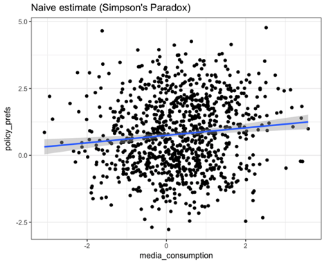
Suppose that, all other things being equal, consuming media causes a slight shift in policy preferences toward the left. But, on average, Republicans consume more news than non-Republicans. And we know that generally Republicans have much more right-leaning preferences.
If we just measure media consumption and policy preferences without including Republicans in the model, we’ll actually estimate that the effect goes in the direction opposite of the true causal effect.
N <- 1000

# Let's say that 40% of people in this population are Republicans
republican <- rbinom(N, 1, .4)

# And they consume more media
media_consumption <- .75 * republican + rnorm(N)

# Consuming more media causes a slight leftward shift in policy
# preferences, and Republicans have more right-leaning preferences
policy_prefs <- -.2 * media_consumption + 2 * republican + rnorm(N)

# for easier plotting later
df <- data.frame(media_consumption, policy_prefs, republican)
df$republican = factor(c("non-republican", "republican")[df$republican + 1])

# If we don't condition on being Republican, we'll actually estimate
# that the effect goes in the *opposite* direction
summary(lm(policy_prefs ~ media_consumption))


Call:
lm(formula = policy_prefs ~ media_consumption)

Residuals:
    Min      1Q  Median      3Q     Max
-3.6108 -0.9559 -0.0198  0.9257  3.9537

Coefficients:
                  Estimate Std. Error t value Pr(>|t|)
(Intercept)        0.68923    0.04323   15.94  < 2e-16 ***
media_consumption  0.15269    0.03966    3.85 0.000126 ***
---
Signif. codes:  0 ‘***’ 0.001 ‘**’ 0.01 ‘*’ 0.05 ‘.’ 0.1 ‘ ’ 1

Residual standard error: 1.317 on 998 degrees of freedom
Multiple R-squared:  0.01463,	Adjusted R-squared:  0.01365
F-statistic: 14.82 on 1 and 998 DF,  p-value: 0.0001257

# Naive plot
qplot(media_consumption, policy_prefs) +
  geom_smooth(method='lm') +
  theme_bw() +
  ggtitle("Naive estimate (Simpson's Paradox)")
The estimate goes in the opposite direction of the true effect! Here’s what the plot looks like:
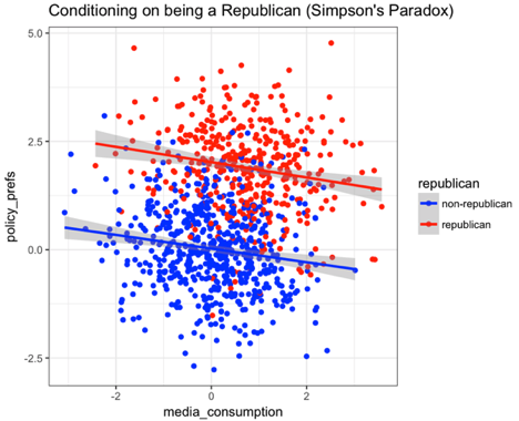
To resolve this paradox, we need to add a factor in the model that indicates whether or not a respondent is a Republican. Adding that factor lets us estimate separate slopes for Republicans and non-Republicans. Note that this is not like estimating an interaction term, where two explanatory variables are multiplied together. It’s not that the slopes are different, we just need to estimate separate ones for Republicans and non-Republicans.
# Condition on being a Republican to get the right estimates
summary(lm(policy_prefs ~ media_consumption + republican))

Call:
lm(formula = policy_prefs ~ media_consumption + republican)

Residuals:
    Min      1Q  Median      3Q     Max
-3.5518 -0.6678 -0.0186  0.6562  3.3009

Coefficients:
                  Estimate Std. Error t value Pr(>|t|)
(Intercept)        0.05335    0.03904   1.366    0.172
media_consumption -0.13615    0.03111  -4.376 1.34e-05 ***
republican         1.93049    0.06758  28.565  < 2e-16 ***
---
Signif. codes:  0 ‘***’ 0.001 ‘**’ 0.01 ‘*’ 0.05 ‘.’ 0.1 ‘ ’ 1

Residual standard error: 0.9774 on 997 degrees of freedom
Multiple R-squared:  0.4581,	Adjusted R-squared:  0.457
F-statistic: 421.4 on 2 and 997 DF,  p-value: < 2.2e-16

# Conditioning on being Republican
qplot(media_consumption, policy_prefs, data=df, colour = republican) +
  scale_color_manual(values = c("blue","red")) +
  geom_smooth(method='lm') +
  theme_bw() +
  ggtitle("Conditioning on being a Republican (Simpson's Paradox)")
Here’s what the plot looks like:
Correlated errors
Another cardinal sin — and one that we should worry a lot about because it often arises from social desirability bias in survey responses — is the phenomenon of correlated errors. This example is inspired by Vavreck (2007).
Here, self-reported turnout and media consumption are caused by a combination of social desirability bias and true turnout and true consumption, respectively:
N <- 1000

# The "Truth"
true_media_consumption <- rnorm(N)
true_vote <- .1 * media_consumption + rnorm(N)

# social desirability bias
social_desirability <- rnorm(N)
#what we actually observe from self reports:
self_report_media_consumption <- true_media_consumption + social_desirability
self_report_vote <- true_vote + social_desirability
Let’s compare the estimated effect sizes of the self-reported data and the “true” data:
# Self reports
summary(lm(self_report_vote ~ self_report_media_consumption))

Call:
lm(formula = self_report_vote ~ self_report_media_consumption)

Residuals:
    Min      1Q  Median      3Q     Max
-3.9604 -0.7766  0.0142  0.8465  4.1811

Coefficients:
                              Estimate Std. Error t value Pr(>|t|)
(Intercept)                    0.02020    0.03951   0.511    0.609
self_report_media_consumption  0.54605    0.02716  20.102   <2e-16 ***
---
Signif. codes:  0 ‘***’ 0.001 ‘**’ 0.01 ‘*’ 0.05 ‘.’ 0.1 ‘ ’ 1

Residual standard error: 1.248 on 998 degrees of freedom
Multiple R-squared:  0.2882,	Adjusted R-squared:  0.2875
F-statistic: 404.1 on 1 and 998 DF,  p-value: < 2.2e-16

# "Truth"
summary(lm(true_vote ~ true_media_consumption))

Call:
lm(formula = true_vote ~ true_media_consumption)

Residuals:
    Min      1Q  Median      3Q     Max
-3.5814 -0.6677 -0.0077  0.6829  3.4799

Coefficients:
                       Estimate Std. Error t value Pr(>|t|)
(Intercept)             0.01372    0.03217   0.426    0.670
true_media_consumption  0.01313    0.03245   0.404    0.686

Residual standard error: 1.017 on 998 degrees of freedom
Multiple R-squared:  0.0001639,	Adjusted R-squared:  -0.000838
F-statistic: 0.1636 on 1 and 998 DF,  p-value: 0.686
The self-reported data is biased toward over-estimating the effect size, a very dangerous problem. How could we fix this? Well, one way is to actually measure social desirability and include it in the model:
summary(lm(self_report_vote ~ self_report_media_consumption + social_desirability))

Call:
lm(formula = self_report_vote ~ self_report_media_consumption +
    social_desirability)

Residuals:
    Min      1Q  Median      3Q     Max
-3.6042 -0.6774 -0.0127  0.6899  3.4470

Coefficients:
                              Estimate Std. Error t value Pr(>|t|)
(Intercept)                    0.01208    0.03220   0.375    0.708
self_report_media_consumption  0.01220    0.03246   0.376    0.707
social_desirability            1.02245    0.04547  22.487   <2e-16 ***
---
Signif. codes:  0 ‘***’ 0.001 ‘**’ 0.01 ‘*’ 0.05 ‘.’ 0.1 ‘ ’ 1

Residual standard error: 1.017 on 997 degrees of freedom
Multiple R-squared:  0.5277,	Adjusted R-squared:  0.5268
F-statistic:   557 on 2 and 997 DF,  p-value: < 2.2e-16
Note that this while most people think about social desirability as being a problem related to measurement error, it is essentially the same problem as omitted variable bias, as described above.
It’s important to remember that omitted variable bias and correlated errors are just two potential problems with regression analysis. Regression models are also not immune to issues associated with low levels of statistical power, the failure to account for the influence of extreme values, and heteroskedasticity, among others. But by simulating the data-generating process, researchers can get a good sense of some of the more common ways in which statistical models might depart from reality.